Here, we will perform an Analysis of Variance (ANOVA) to determine if there are any statistically significant differences between the means of three or more independent groups.
Comparison of means of three samples
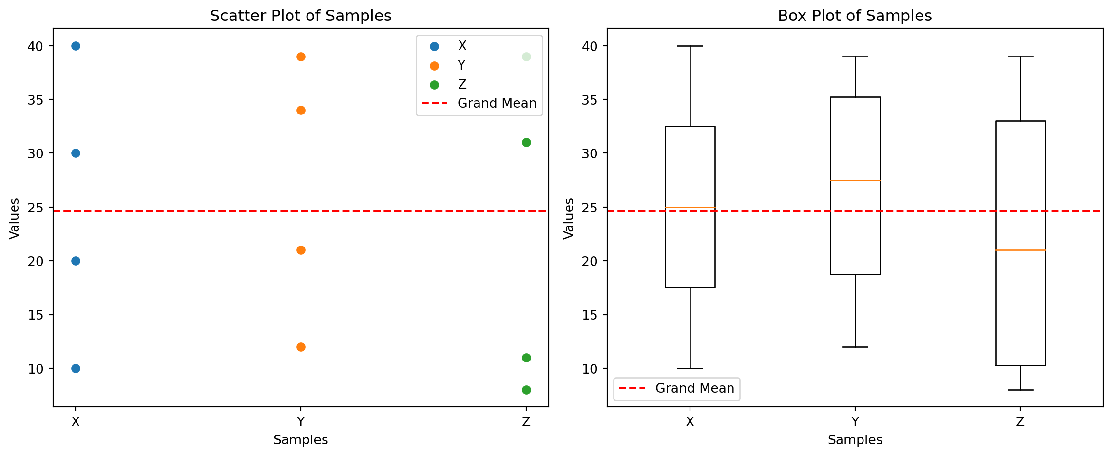
Consider three independent samples:
X: 10, 20, 30, 40
Y: 12, 21, 34, 39
Z: 8, 11, 31, 39
We want to test if the means of these three samples are significantly different from each other.
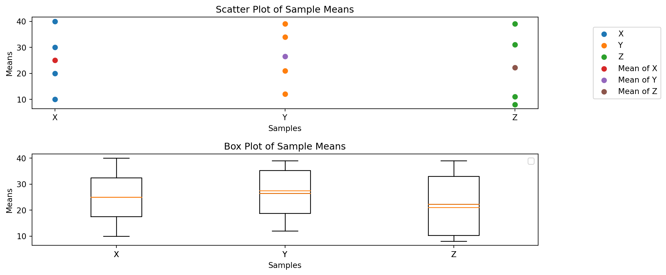
Calculate the mean of each sample:
Mean of X: \((10 + 20 + 30 + 40) / 4 = 25\)
Mean of Y: \((12 + 21 + 34 + 39) / 4 = 26.5\)
Mean of Z: \((8 + 11 + 31 + 39) / 4 = 22.25\)
Calculate the overall mean (grand mean) of all the samples combined:
import numpy as npimport matplotlib.pyplot as plt# DataX = np.array([10, 20, 30, 40])Y = np.array([12, 21, 34, 39])Z = np.array([8, 11, 31, 39])# Grand meangrand_mean = np.mean(np.concatenate([X, Y, Z]))# Scatter plotplt.figure(figsize=(12, 5))plt.subplot(1, 2, 1)plt.scatter(np.ones_like(X), X, label='X')plt.scatter(np.ones_like(Y) *2, Y, label='Y')plt.scatter(np.ones_like(Z) *3, Z, label='Z')plt.xticks([1, 2, 3], ['X', 'Y', 'Z'])plt.xlabel('Samples')plt.ylabel('Values')plt.title('Scatter Plot of Samples')plt.axhline(grand_mean, color='red', linestyle='--', label='Grand Mean')plt.legend()# Box plotplt.subplot(1, 2, 2)plt.boxplot([X, Y, Z], labels=['X', 'Y', 'Z'])plt.xlabel('Samples')plt.ylabel('Values')plt.title('Box Plot of Samples')plt.axhline(grand_mean, color='red', linestyle='--', label='Grand Mean')plt.legend()plt.tight_layout()plt.show()
import numpy as npimport matplotlib.pyplot as plt# DataX = np.array([10, 20, 30, 40])Y = np.array([12, 21, 34, 39])Z = np.array([8, 11, 31, 39])# Meansmean_X = np.mean(X)mean_Y = np.mean(Y)mean_Z = np.mean(Z)# Grand meangrand_mean = np.mean(np.concatenate([X, Y, Z]))# Scatter plotplt.figure(figsize=(12, 5))plt.subplot(2, 1, 1)plt.scatter(np.ones_like(X), X, label='X')plt.scatter(np.ones_like(Y) *2, Y, label='Y')plt.scatter(np.ones_like(Z) *3, Z, label='Z')plt.scatter([1], [mean_X], label='Mean of X')plt.scatter([2], [mean_Y], label='Mean of Y')plt.scatter([3], [mean_Z], label='Mean of Z')plt.xticks([1, 2, 3], ['X', 'Y', 'Z'])plt.xlabel('Samples')plt.ylabel('Means')plt.title('Scatter Plot of Sample Means')#plt.axhline(grand_mean, color='red', linestyle='--', label='Grand Mean')#plt.legend(outside)plt.legend(loc='center right', bbox_to_anchor=(1.25, 0.5))# Box plotplt.subplot(2, 1, 2)plt.boxplot([X, Y, Z], labels=['X', 'Y', 'Z'])plt.boxplot([[mean_X], [mean_Y], [mean_Z]], labels=['X', 'Y', 'Z'])plt.xlabel('Samples')plt.ylabel('Means')plt.title('Box Plot of Sample Means')#plt.axhline(grand_mean, color='red', linestyle='--', label='Grand Mean')plt.legend()plt.tight_layout()plt.show()
No artists with labels found to put in legend. Note that artists whose label start with an underscore are ignored when legend() is called with no argument.
4.2 One-way Analysis of Variance
Consider m independent samples, each of size n.
The members of the ith sample are denoted as: \(X_{i1}, X_{i2}, \dots, X_{in}\).
To estimate the m unknown parameters\(\mu_1, \dots, \mu_m\):
Let \(X_{i}\) denote the sample mean of the ith sample: \[
\bar{X}_{i} = \sum_{j=1}^{n} \frac{X_{ij}}{n}
\]
Here, \(\bar{X}_{i}\) is the estimator of the population mean \(\mu_i\) for \(i = 1, \dots, m\).
Substituting the estimators \(\bar{X}_{i}\) for \(\mu_i\) in Equation Equation 4.1:
The resulting variable: \[
\sum_{i=1}^{m} \sum_{j=1}^{n} \frac{(X_{ij} - \bar{X}_{i})^2}{\sigma^2}
\tag{4.2}\] follows a chi-square distribution with nm − m degrees of freedom.
(One degree of freedom is lost for each estimated parameter.)
We thus have our first estimator of \(\sigma^2\), namely, SSW /(nm - m). The statistic SSW is called the Sum of Squares Within Samples aka ( within samples sum of squares or sum of squares within groups).
Also, note that this estimator was obtained without assuming anything about the truth or falsity of the null hypothesis.
Our second estimator of \(\sigma^2\) is valid only when the null hypothesis is true.
Assume \(H_0\) is true, meaning all population means \(\mu_i\) are equal, i.e., \(\mu_i = \mu\) for all \(i\).
Under this assumption:
The sample means \(\bar{X}_1, \bar{X}_2, \dots, \bar{X}_m\) are normally distributed with:
Mean: \(\mu\).
Variance: \(\frac{\sigma^2}{n}\).
We have; \[
\frac{\bar{X}_{i.} - \mu}{\sqrt{\sigma^2/n}} = \frac{\sqrt{n}(\bar{X}_{i.} - \mu)}{\sigma}
\] follows a standard normal distribution; hence, \[
n \sum_{i=1}^{m} \frac{(\bar{X}_{i.} - \mu)^2}{\sigma^2} \sim \chi^2_m
\tag{4.3}\] follows a chi-square distribution with m degrees of freedom when \(H_0\) is true.
When all population means are equal to \(\mu\), the estimator of \(\mu\) is the average of all nm data values, denoted as \(\bar{X}_{..}\): \[
\bar{X}_{..} = \frac{\sum_{i=1}^{m} \sum_{j=1}^{n} X_{ij}}{nm} = \frac{\sum_{i=1}^{m} \bar{X}_{i.}}{m}
\]
Substituting \(\bar{X}_{..}\) for the unknown parameter \(\mu\) in Equation 4.3:
When \(H_0\) is true, the resulting quantity: \[
n \sum_{i=1}^{m} \frac{(\bar{X}_{i.} - \bar{X}_{..})^2}{\sigma^2}
\]
The resulting quantity: \[
n \sum_{i=1}^{m} \frac{(\bar{X}_{i.} - \bar{X}_{..})^2}{\sigma^2}
\] will be a chi-square random variable with m - 1 degrees of freedom.
\(\frac{SSb}{m-1}\) estimates \(\sigma^2\) when \(H_0\) is true.
Because it can be shown that \(\frac{SSb}{m-1}\) will tend to exceed \(\sigma^2\) when \(H_0\) is not true, now it is reasonable to let the test statistic be given by
and to reject \(H_0\) when \(TS\) is sufficiently large.
How to do the hypothesis testing
To determine how large \(TS\) needs to be to justify rejecting \(H_0\), we use the fact that:
If \(H_0\) is true, then \(SSb\) and \(SSW\) are independent.
It follows that, when \(H_0\) is true, \(TS\) has an \(F\)-distribution with \(m-1\) numerator and \(nm-m\) denominator degrees of freedom.
Let \(F_{m-1,nm-m,\alpha}\) denote the \(100(1-\alpha)\) percentile of this distribution — that is, \(P\{F_{m-1,nm-m} > F_{m-1,nm-m,\alpha}\} = \alpha\).
We use the notation \(F_{r,s}\) to represent an \(F\)-random variable with \(r\) numerator and \(s\) denominator degrees of freedom.
The significance level \(\alpha\) test of \(H_0\) is as follows:
Reject \(H_0\) if \(\frac{\frac{SSb}{m-1} }{ \frac{SSW}{nm-m}} > F_{m-1,nm-m,\alpha}\).
Do not reject \(H_0\), otherwise.
Note
The following algebraic identity, known as the sum of squares identity, is useful for simplifying computations, especially when done by hand:
The Sum of Squares Identity: \[
\sum_{i=1}^{m} \sum_{j=1}^{n} X_{ij}^2 = nm \bar{X}_{..}^2 + SSb + SSW
\]
Here:
\(\sum_{i=1}^{m} \sum_{j=1}^{n} X_{ij}^2\) represents the total sum of squares of all observations.
\(nm \bar{X}_{..}^2\) is the contribution from the grand mean (\(\bar{X}_{..}\)).
\(SSb\) (Sum of Squares Between) measures the variation between sample means.
\(SSW\) (Sum of Squares Within) measures the variation within each sample.
This identity helps decompose the total variability in the data into components that can be analyzed separately.
When performing calculations by hand, the quantity SSb (Sum of Squares Between) should be computed first. It is defined as: \[
SSb = n \sum_{i=1}^{m} (\bar{X}_{i.} - \bar{X}_{..})^2
\]
Once SSb has been calculated, SSW (Sum of Squares Within) can be determined using the sum of squares identity. To do this:
Compute the total sum of squares: \[
\sum_{i=1}^{m} \sum_{j=1}^{n} X_{ij}^2
\]
Compute the term involving the grand mean: \[
nm \bar{X}_{..}^2
\]
Use the sum of squares identity to find SSW: \[
SSW = \sum_{i=1}^{m} \sum_{j=1}^{n} X_{ij}^2 - nm \bar{X}_{..}^2 - SSb
\]
This approach simplifies the computation process by breaking it into manageable steps and leveraging the sum of squares identity.
Alternative Method
Another useful identity involving the sum of squares is:
Error Sum of Squares (\(SS_{total}\)): \(SS_{total}=SSb + SSW\)
where Total Sum of Squares (\(SS_{total}\)): \(SS_{total}=\sum_{i=1}^m\sum_{j=1}^n(X_{ij}-\bar{X}_{..})^2\)
This identity can also be used for the anova analysis while performing the computations by hand.
This approach too simplifies the computation process by breaking it into manageable steps and leveraging the sum of squares identity.
Summary of one-way analysis of variance
\[
\begin{array}{|c|c|c|}
\hline
\textbf{Source of Variation} & \textbf{Sum of Squares} & \textbf{Degrees of Freedom} \\
\hline
\text{Between samples} & SS_b = n \sum_{i=1}^m (\bar{X}_{i.} - \bar{X}_{..})^2 & m - 1 \\
\hline
\text{Within samples} & SS_W = \sum_{i=1}^m \sum_{j=1}^n (X_{ij} - \bar{X}_{i.})^2 & nm - m \\
\hline
\end{array}
\]
Value of Test Statistic, \(TS = \frac{SS_b/(m-1)}{SS_W/(nm-m)}\)
Significance level \(\alpha\) test:
reject \(H_0\) if \(TS \geq F_{m-1,nm-m,\alpha}\)
do not reject otherwise
If \(TS = v\), then \(p\)-value = \(P\{F_{m-1,nm-m} \geq v\}\)
Problem
An auto rental firm is using 15 identical motors that are adjusted to run at a fixed speed to test 3 different brands of gasoline. Each brand of gasoline is assigned to exactly 5 of the motors. Each motor runs on 10 gallons of gasoline until it is out of fuel. The following data represents the total mileages achieved by different motors using three types of gas:
Gas 1: \(220, 251, 226, 246, 260\)
Gas 2: \(244, 235, 232, 242, 225\)
Gas 3: \(252, 272, 250, 238, 256\)
Test the hypothesis that the average mileage is not affected by the type of gas used. (In other words, determine if there is a significant difference in the mean mileages for the three types of gas.)
Multiple Comparisons of Sample Means
When the null hypothesis of equal means is rejected, we are often interested in comparing the different sample means \(\mu_1, \dots, \mu_m\).
One commonly used procedure for this purpose is known as the T-method.
For a specified significance level \(\alpha\), this method provides joint confidence intervals for all \(\binom{m}{2}\) differences \(\mu_i - \mu_j\) (where \(i \neq j\), and \(i, j = 1, \dots, m\)), ensuring that with probability \(1 - \alpha\), all confidence intervals will contain their respective differences \(\mu_i - \mu_j\).
The T-method is based on the following result:
With probability \(1 - \alpha\), for every \(i \neq j\): \[
X_{i.} - X_{j.} - W < \mu_i - \mu_j < X_{i.} - X_{j.} + W
\]
Where: - \(X_{i.}\) and \(X_{j.}\) are the sample means for groups \(i\) and \(j\), respectively. - \(W\) is the critical value derived from the Studentized range distribution, adjusted for multiple comparisons.
where \[
W = \sqrt{\frac{1}{n}} \cdot C(m, nm - m, \alpha) \cdot \sqrt{\frac{SSW}{(nm - m)}}
\] and the values of \(C(m, nm - m, \alpha)\) are provided for \(\alpha = 0.05\) and \(\alpha = 0.01\).
Problem
A college administrator claims that there is no difference in first-year grade point averages for students entering the college from any of three different city high schools. The following data provide the first-year grade point averages of 12 randomly chosen students, 4 from each of the three high schools. At the 5 percent level of significance, do these data disprove the administrator’s claim? If so, determine confidence intervals for the difference in means of students from the different high schools, such that we can be 95 percent confident that all of the interval statements are valid.
School 1: 3.2, 3.4, 3.3, 3.5 School 2: 3.4, 3.0, 3.7, 3.3 School 3: 2.8, 2.6, 3.0, 2.7
4.2.1 One-Way Analysis of Variance with Unequal Sample Sizes
\[
\begin{array}{|c|c|c|}
\hline
\textbf{Source of Variation} & \textbf{Sum of Squares} & \textbf{Degrees of Freedom} \\
\hline
\text{Between samples} & SS_b = \sum_{i=1}^m n_i (\bar{X}_{i.} - \bar{X}_{..})^2 & m - 1 \\
\hline
\text{Within samples} & SS_W = \sum_{i=1}^m \sum_{j=1}^n (X_{ij} - \bar{X}_{i.})^2 & N - m \\
\hline
\end{array}
\]
where, N = \(\sum_{i=1}^m n_i\)
Value of Test Statistic, \(TS = \frac{SS_b/(m-1)}{SS_W/(N-m)}\)
Significance level \(\alpha\) test:
reject \(H_0\) if \(TS \geq F_{m-1,N-m,\alpha}\)
do not reject otherwise
If \(TS = v\), then \(p\)-value = \(P\{F_{m-1,N-m} \geq v\}\)
Problem
Test the hypothesis that the following three independent samples are drawn from the same normal probability distribution.
Use a statistical test to determine whether the means of these samples are significantly different.
4.3 Two-way Analysis of Variance
Introduction
Example
Consider that four different examinations were administered to each of 5 students, with the scores shown in the table below. Each of the 20 data points is influenced by two factors: the exam and the student whose score on that exam is being recorded.
In general, suppose there are m possible levels of the first factor (row factor) and n possible levels of the second factor (column factor). Let \(X_{ij}\) denote the value obtained when:
Here, the first factor is referred to as the row factor, and the second factor is referred to as the column factor.
As in the case of one-way analysis assume that the data \(X_{ij}\) (\(i = 1, \dots, m\), \(j = 1, \dots, n\)) are independent normal random variables with a common variance \(\sigma^2\). However, unlike the one-way analysis, where only a single factor affected the mean value of a data point, we now assume that the mean value of the data depends additively on both its row and column factors.
Row Mean (\(\bar{X}_i.\)): \[
\bar{X}_{i.} = \frac{\sum_{j=1}^n X_{ij}}{n} = \text{Average of the values in row } i
\]
Column Mean (\(\bar{X}_{.j}\)): \[
\bar{X}_{.j} = \frac{\sum_{i=1}^m X_{ij}}{m} = \text{Average of the values in column } j
\]
Grand Mean (\(\bar{X}_{..}\)): \[
\bar{X}_{..} = \frac{\sum_{i=1}^m \sum_{j=1}^n X_{ij}}{nm} = \text{Average of all data values}
\]
Problem 1
A researcher aims to investigate the impact of two factors on crop yield:
Factor A (Fertilizer Type): Two levels - Type 1 (\(T1\)) and Type 2 (\(T2\)).
Factor B (Irrigation Level): Three levels - Low (\(L\)), Medium (\(M\)), and High (\(H\)).
The researcher measures the yield (in kg) for each combination of factors. Due to the high cost of the experiment, only one observation is recorded for each combination. The data is as follows:
Fertilizer
Irrigation
Yield (kg)
Type 1 (\(T1\))
Low (\(L\))
55
Type 1 (\(T1\))
Medium (\(M\))
60
Type 1 (\(T1\))
High (\(H\))
70
Type 2 (\(T2\))
Low (\(L\))
55
Type 2 (\(T2\))
Medium (\(M\))
65
Type 2 (\(T2\))
High (\(H\))
75
Note
Here also we have an useful identity for the sum of squares
Total Sum of Squares (\(SS_{total}\)): \(SS_{total}=SS_{error}+SS_r+SS_c\)
where Total Sum of Squares (\(SS_{total}\)): \(SS_{total}=\sum_{i=1}^m\sum_{j=1}^n(X_{ij}-\bar{X}_{..})^2\)
Supplementary Topics
Degrees of Freedom (dof)
The statement “One degree of freedom is lost for each estimated parameter” is a key concept in statistics, especially in hypothesis testing and parameter estimation. Here’s a detailed explanation:
What Are Degrees of Freedom?
Degrees of freedom (df) represent the number of independent pieces of information available to estimate a parameter or test a hypothesis.
In simpler terms, it’s the number of values in a calculation that are free to vary after certain constraints (like estimating parameters) are applied.
Why Are Degrees of Freedom Lost?
When you estimate parameters (e.g., population means, variances) from sample data, you use the data itself to calculate these estimates.
Each time you estimate a parameter, you impose a constraint on the data, reducing the number of independent pieces of information available.
Example: If you estimate the sample mean (\(\bar{X}\)) from a dataset, you use the data to calculate \(\bar{X}\). This means one piece of information (one degree of freedom) is “used up” in estimating \(\bar{X}\), and the remaining data points are no longer fully independent.
Application in the Context of the Problem
In the given problem:
You have m samples, each of size n, and you estimate the mean of each sample (\(\mu_i\)) using the sample mean (\(\bar{X}_{i.}\)).
Each time you estimate a mean (\(\mu_i\)), you lose one degree of freedom because the data is used to calculate that estimate.
Since you estimate m means (\(\mu_1, \mu_2, \dots, \mu_m\)), you lose m degrees of freedom in total.
Mathematical Explanation
Initially, the sum of squares: \[
\sum_{i=1}^{m} \sum_{j=1}^{n} \frac{(X_{ij} - \mu_i)^2}{\sigma^2}
\] follows a chi-square distribution with nm degrees of freedom (since there are nm independent observations).
However, when you replace the true means (\(\mu_i\)) with their estimates (\(\bar{X}_{i.}\)), you lose m degrees of freedom (one for each estimated mean). This is because the estimates are derived from the data, reducing the independence of the observations.
As a result, the modified sum of squares: \[
\sum_{i=1}^{m} \sum_{j=1}^{n} \frac{(X_{ij} - \bar{X}_{i.})^2}{\sigma^2}
\] follows a chi-square distribution with nm - m degrees of freedom.
Why Does This Matter?
Degrees of freedom affect the shape and critical values of the chi-square distribution, which is used for hypothesis testing.
Losing degrees of freedom accounts for the fact that estimating parameters introduces uncertainty into the analysis.
This adjustment ensures that statistical tests (e.g., ANOVA) are accurate and reliable.
Summary
Degrees of freedom represent independent information in the data.
Each estimated parameter (e.g., a mean) reduces the degrees of freedom by 1 because the data is used to calculate the estimate.
In the problem, estimating m means reduces the degrees of freedom from nm to nm - m, ensuring the chi-square distribution is correctly applied.