2  Parameter Estimation

2.1 Point Estimation: Maximum Likelihood Estimators

(Please refer the book titled “Introduction to Probability and Statistics for Engineers and Scientists” by Sheldon M Ross for more details)

2.2 Interval Estimates

• Consider a sample \(X_1, X_2, \ldots, X_n\) drawn from a known distribution with an unknown mean \(\mu\).

• It is established that the sample mean \(\bar{X} = \frac{1}{n} \sum_{i=1}^{n} X_i\) serves as the maximum likelihood estimator for \(\mu\).

• However, the sample mean \(\bar{X}\) is not expected to be exactly equal to \(\mu\), but rather close to it.

• Therefore, instead of providing a single point estimate, it is often more useful to specify an interval within which we are confident that \(\mu\) lies.

• To determine such an interval estimator, we utilize the probability distribution of the point estimator.

2.2.1 Confidence Intervals for the Mean of a normal population with known Variance

• Consider a sample \(X_1, X_2, \ldots, X_n\) drawn from a normal distribution with an unknown mean \(\mu\) and a known variance \(\sigma^2\).

• The point estimator \(\bar{X}\) is normal with mean \(\mu\) and variance \(\sigma^2\)/n.

• Therefore, \(\frac{\bar{X} - \mu}{\sigma/\sqrt{n}}\) follows a standard normal distribution.

What to do

Consider that I want to find an interval around \(\bar{X}\) such that the actual population mean \(\mu\) falls within the interval, say 95 % of the times.

Tip

• For finding such an interval, I can use the Z-table. From the Z-table I can find:

\[ P\left( -1.96 < \frac{\bar{X} -\mu}{\sigma/\sqrt{n}} < 1.96 \right) = 0.9750 - 0.0250 = 0.95 \]

• Rewriting the above equation:

\[ P\left( -1.96\frac{\sigma}{\sqrt{n}} < \bar{X} -\mu < 1.96\frac{\sigma}{\sqrt{n}}\right) = 0.95 \]

\[ P\left( 1.96\frac{\sigma}{\sqrt{n}} > \mu - \bar{X} > -1.96\frac{\sigma}{\sqrt{n}}\right) = 0.95 \]

\[ P\left( -1.96\frac{\sigma}{\sqrt{n}} < \mu - \bar{X} < 1.96\frac{\sigma}{\sqrt{n}} \right) = 0.95 \]

\[ P\left( \bar{X} - 1.96\frac{\sigma}{\sqrt{n}} < \mu < \bar{X} + 1.96\frac{\sigma}{\sqrt{n}}\right) = 0.95 \]

• We have P(Z < -1.96) = 0.025, similarly P(Z > 1.96) = 0.025. Usually 1.96 is represented generally as \(z_{0.025}\). Thus, P(Z < -z\(_{0.025}\)) = 0.025 and P(Z > z\(_{0.025}\)) = 0.025.

• Hence, 100(1-0.05) percent confidence interval for the mean of a normal population with known variance is:

\[ P\left( \bar{X} - z_{0.025}\frac{\sigma}{\sqrt{n}} < \mu < \bar{X} + z_{0.025}\frac{\sigma}{\sqrt{n}}\right) = 0.95 \]

\[ P\left( \bar{X} - z_{0.05/2}\frac{\sigma}{\sqrt{n}} < \mu < \bar{X} + z_{0.05/2}\frac{\sigma}{\sqrt{n}}\right) = (1 - 0.05) \]

• For a confidence level of \(100(1-\alpha)\) percent, the corresponding critical value from the standard normal distribution is \(z_{\alpha/2}\).

• The \(100(1-\alpha)\) percent confidence interval for \(\mu\) is given by:

\[ \mu \in \left( \bar{X} - z_{\alpha/2} \frac{\sigma}{\sqrt{n}}, \bar{X} + z_{\alpha/2} \frac{\sigma}{\sqrt{n}} \right) \tag{2.1}\]

• The interval as given in Equation 2.1 is called a two-sided confidence interval.

• Also the term \(z_{\alpha/2} \frac{\sigma}{\sqrt{n}}\) is called the margin of error.

Derivation of two-sided confidence interval

• To find 100(1-\(\alpha\)) percent confidence interval of mean (\(\mu\)), we have;

\[ P\left( -z_{\alpha/2} < \frac{\bar{X} -\mu}{\sigma/\sqrt{n}} < z{_\alpha/2} \right) = 1 - \alpha \]

• Doing the same manipulations we did earlier for obtaining the 95percent confidence interval we can obtain:

\[ P\left( \bar{X} - z_{\alpha/2} \frac{\sigma}{\sqrt{n}} < \mu < \bar{X} - z_{\alpha/2} \frac{\sigma}{\sqrt{n}} \right) = 1 - \alpha \]

• The above equation give us the required confidence interval, as given in Equation 2.1.

What if !?

What if we are interested in one sided confidence intervals !!?

One-sided Upper Confidence Iterval

• To determine such an interval, for a standard normal random variable Z, we have;

\[ P\left( Z < 1.645 \right) = 0.95 \]

• Thus, \[ P\left( \frac{\bar{X} - \mu}{\sigma/\sqrt{n}} < 1.645 \right) = 0.95 \]

\[ P\left( \mu -\bar{X} > - 1.645\frac{\sigma}{\sqrt{n}} \right) = 0.95 \]

\[ P\left( \mu > \bar{X} - 1.645\frac{\sigma}{\sqrt{n}} \right) = 0.95 \]

• Thus a 95 percent one-sided upper confidence interval for \(\mu\) is

\[ \mu \in \left( \bar{X} - 1.645\frac{\sigma}{\sqrt{n}}, \infty \right) \]

or in other words; 100(1-0.05) percent one-sided upper confidence interval for \(\mu\) is

\[ \mu \in \left( \bar{X} - z_{0.05}\frac{\sigma}{\sqrt{n}}, \infty \right) \]

Oneside interval!

Can you think of another one sided confidence interval?

One-sided lower confidence interval

• We have \[ P\left( Z > - 1.645 \right) = 0.95 \]

• Proceed just like in the previous case and you will find a 100(1-0.05) percent one-sided lower confidence interval for \(\mu\) as;

\[ \mu \in \left( -\infty, \bar{X} + z_{0.05}\frac{\sigma}{\sqrt{n}} \right) \]

• In general, 100(1-\(\alpha\)) percent one-sided upper confidence interval for \(\mu\) is given in Equation 2.2.

\[ \mu \in \left( \bar{X} - z_{\alpha}\frac{\sigma}{\sqrt{n}}, \infty \right) \tag{2.2}\]

• Also, 100(1-\(\alpha\))percent one-sided lower confidence interval for \(\mu\) is given in Equation 2.3. \[ \mu \in \left( -\infty, \bar{X} + z_{\alpha}\frac{\sigma}{\sqrt{n}} \right) \tag{2.3}\]

• The python code below creates a sample and find 95% confidence interval for the mean if the population standard deviation is assumed to be 10. Other values are specified in the code.

import numpy as np
import matplotlib.pyplot as plt

# Parameters
mu = 50  # true mean
sigma = 10  # known standard deviation
n = 30  # sample size
alpha = 0.05  # significance level

# Generate a sample
np.random.seed(0)
sample = np.random.normal(mu, sigma, n)
sample_mean = np.mean(sample)

# Calculate the confidence interval
z = 1.96  # z-value for 95% confidence
margin_of_error = z * (sigma / np.sqrt(n))
confidence_interval = (sample_mean - margin_of_error, sample_mean + margin_of_error)

# Plot the sample and confidence interval
plt.figure(figsize=(8, 4))
plt.hist(sample, bins=10, alpha=0.7, color='blue', edgecolor='black')
plt.axvline(sample_mean, color='red', linestyle='dashed', linewidth=2, label='Sample Mean')
plt.axvline(confidence_interval[0], color='green', linestyle='dashed', linewidth=2, label='95% CI Lower Bound')
plt.axvline(confidence_interval[1], color='green', linestyle='dashed', linewidth=2, label='95% CI Upper Bound')
plt.title('Sample Distribution with 95% Confidence Interval')
plt.xlabel('Value')
plt.ylabel('Frequency')
plt.legend()
plt.show()

print(f"Sample Mean: {sample_mean}")
print(f"95% Confidence Interval: {confidence_interval}")

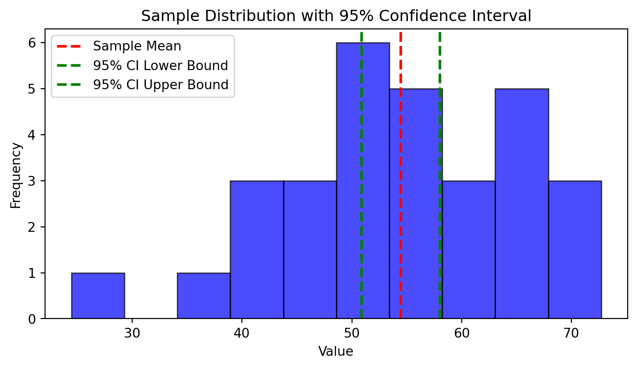
Sample Mean: 54.42856447263174
95% Confidence Interval: (50.85011043026466, 58.007018514998826)

Problem

Suppose that when a signal having value \(\mu\) is transmitted from location A the value received at location B is normally distributed with mean \(\mu\) and variance 4. That is, if \(\mu\) is sent, then the value received is \(\mu\) + N where N, representing noise, is normal with mean 0 and variance 4. To reduce error, suppose the same value is sent 9 times. If the successive values received are 5, 8.5, 12, 15, 7, 9, 7.5, 6.5, 10.5;

(a). construct a 95 percent two-sided confidence interval for \(\mu\).

(b). construct 95 percent one-sided upper and lower confidence intervals for \(\mu\).

Problem

Suppose a quality control manager at a factory wants to ensure that the average weight of a product is at least 500 grams. They take a random sample of 30 products and find the sample mean weight to be 495 grams with a standard deviation of 10 grams. Help the manager to estimate the minimum average weight of the products with 95% confidence.

2.2.2 Confidence Intervals for the Mean of a normal population with unknown Variance

• If you recollect the discussion we had about the sample mean from a normal population with unknown variance we saw that variable t\(_{n-1}\) given by:

\[ t_{n-1} = \sqrt{n}\frac{\bar{X} - \mu}{S} \]

has a t-distribution with n-1 degrees of freedom.

• Because of the symmetry of the t-distribution we can write for any \(\alpha\) \(\in\) (0, 1/2);

\[ P\left( -t_{\alpha/2, n-1} < \sqrt{n}\frac{\bar{X} - \mu}{S} < t_{\alpha/2, n-1} \right) = 1 - \alpha \]

\[ P\left( -\bar{X} - t_{\alpha/2, n-1} \frac{\sqrt{n}}{S} < - \mu < -\bar{X} + t_{\alpha/2, n-1} \frac{\sqrt{n}}{S} \right) = 1 - \alpha \]

\[ P\left( \bar{X} + t_{\alpha/2, n-1} \frac{\sqrt{n}}{S} > \mu > \bar{X} - t_{\alpha/2, n-1} \frac{\sqrt{n}}{S} \right) = 1 - \alpha \]

\[ P\left( \bar{X} - t_{\alpha/2, n-1} \frac{S}{\sqrt{n}} < \mu < \bar{X} + t_{\alpha/2, n-1} \frac{S}{\sqrt{n}} \right) = 1 - \alpha \]

• If the sample mean is \(\bar{X}\) and sample standard deviation S, then we can say that with 100(1-\(\alpha\)) percent confidence that

\[ \mu \in \left(\bar{X} - t_{\alpha/2, n-1} \frac{S}{\sqrt{n}}, \bar{X} + t_{\alpha/2, n-1} \frac{S}{\sqrt{n}} \right) \]

• In this case 100(1-\(\alpha\)) percent one-sided upper confidence interval can be obtained from the fact that:

\[ P\left( \sqrt{n}\frac{(\bar{X} - \mu)}{S} < t_{\alpha, n-1}\right) = 1 - \alpha \]

\[ P\left( \mu > \bar{X} - \frac{S}{\sqrt{n}} t_{\alpha, n-1} \right) = 1 - \alpha \]

• Thus 100(1 − \(\alpha\)) percent one-sided upper confidence interval for the mean in this case is given by;

\[ \mu \in \left( \bar{X} - \frac{S}{\sqrt{n}} t_{\alpha, n-1}, \infty \right) \]

• Thus 100(1 − \(\alpha\)) percent one-sided lower confidence interval for the mean in this case is given by;

\[ \mu \in \left( -\infty, \bar{X} + \frac{S}{\sqrt{n}} t_{\alpha, n-1} \right) \]

Problem

Let us again consider the previous problem but let us now suppose that when the value \(\mu\) is transmitted at location A then the value received at location B is normal with mean \(\mu\) and variance \(\sigma^2\) but with \(\sigma^2\) being unknown. If 9 successive values are, 5, 8.5, 12, 15, 7, 9, 7.5, 6.5, and 10.5, compute a 95 percent confidence interval for \(\mu\).

2.2.3 Confidence Intervals for the Variance of a Normal Distribution

• If we are sampling from a normal distribution with unknown mean and unknown variance then;

\[ (n-1) \frac{S^2}{\sigma^2} \sim \chi^2_{n-1} \]

follows a chi-squared distribution.

• We have

\[ P\left( \chi^2_{1-\alpha/2, n-1} \leq (n-1)\frac{S^2}{\sigma^2} \leq \chi^2_{\alpha/2, n-1} \right) = 1 - \alpha \]

\[ P\left( \chi^2_{1-\alpha/2, n-1} \leq (n-1)\frac{S^2}{\sigma^2} \leq \chi^2_{\alpha/2, n-1} \right) = 1 - \alpha \]

\[ P\left( \frac{(n-1)S^2}{\chi^2_{\alpha/2, n-1}} \leq \sigma^2 \leq \frac{(n-1)S^2}{\chi^2_{1-\alpha/2, n-1}} \right) = 1 - \alpha \]

• Hence, 100(1-\(\alpha\)) percent two-sided confidence interval for the variance in this case;

\[ \sigma^2 \in \left( \frac{(n-1)S^2}{\chi^2_{\alpha/2, n-1}}, \frac{(n-1)S^2}{\chi^2_{1-\alpha/2, n-1}} \right) \]

• The 100(1-\(\alpha\)) percent one-sided upper and lower confidence intervals in this case will be respectively;

\[ \left(\frac{(n-1)S^2}{\chi^2_{\alpha, n-1}}, \infty \right) \]

and

\[ \left( 0, \frac{(n-1)S^2}{\chi^2_{1-\alpha, n-1}} \right) \]

Problem

A standardized procedure is expected to produce washers with very small deviation in their thicknesses. Suppose that 10 such washers were chosen and measured. If the thicknesses of these washers were, in inches; .123, .133, .124, .125, .126, .128, .120, .124, .130, and .126. What is a 90 percent confidence interval for the standard deviation of the thickness of a washer produced by this procedure?

All problems and most part of text are taken from Ross (2009) .

Ross, Sheldon. 2009. “Probability and Statistics for Engineers and Scientists.” Elsevier, New Delhi 16: 32–33.