Many engineering and scientific problems aim to determine relationships between variables.
Example: In a chemical process, the relationship between output, temperature, and catalyst amount is of interest.
Knowing this relationship allows predicting outputs for different temperature and catalyst values.
Typically, there is a single response variable\(Y\) (dependent variable) that depends on a set of input variables\(x_1, x_2, \dots, x_r\) (independent variables).
The simplest relationship between \(Y\) and \(x_1, x_2, \dots, x_r\) is a linear relationship: \[
Y = \beta_0 + \beta_1 x_1 + \beta_2 x_2 + \dots + \beta_r x_r
\tag{5.1}\]
Here, \(\beta_0, \beta_1, \dots, \beta_r\) are constants.
In practice, exact predictions are rarely possible due to random errors.
The relationship is better expressed as: \[
Y = \beta_0 + \beta_1 x_1 + \beta_2 x_2 + \dots + \beta_r x_r + e
\tag{5.2}\]
\(e\) represents the random error, assumed to have a mean of \(0\).
Alternatively, the relationship can be expressed in terms of the expected value: \[
E[Y \mid \mathbf{x}] = \beta_0 + \beta_1 x_1 + \beta_2 x_2 + \dots + \beta_r x_r
\]
\(\mathbf{x} = (x_1, x_2, \dots, x_r)\) is the set of independent variables.
\(E[Y \mid \mathbf{x}]\) is the expected response given the inputs \(\mathbf{x}\).
The Equation 5.2 is called a linear regression equation.
It describes the regression of \(Y\) on the independent variables \(x_1, x_2, \dots, x_r\).
The quantities \(\beta_0, \beta_1, \dots, \beta_r\) are called regression coefficients, and must usually be estimated from a set of data.
A regression equation can be classified based on the number of independent variables:
Simple regression equation: Contains a single independent variable (\(r = 1\)).
Multiple regression equation: Contains many independent variables.
A simple linear regression model assumes a linear relationship between the mean response and a single independent variable.
It is expressed as: \[
Y = \alpha + \beta x + e
\]
\(x\) is the value of the independent variable (also called the input level).
\(Y\) is the response.
\(e\) represents the random error, assumed to be a random variable with mean \(0\).
Regression analysis is used to find the mean value of the dependent variable \(Y\) given the independent variables \(\mathbf{x}\).
The mean value of \(Y\) given \(\mathbf{x}\) is denoted as \(E[Y \mid \mathbf{x}]\).
By estimating the regression coefficients \(\beta_0, \beta_1, \dots, \beta_r\), we can predict the mean response for any given set of input variables.
This is particularly useful in understanding the central tendency of the response variable and making informed decisions based on the predicted mean.
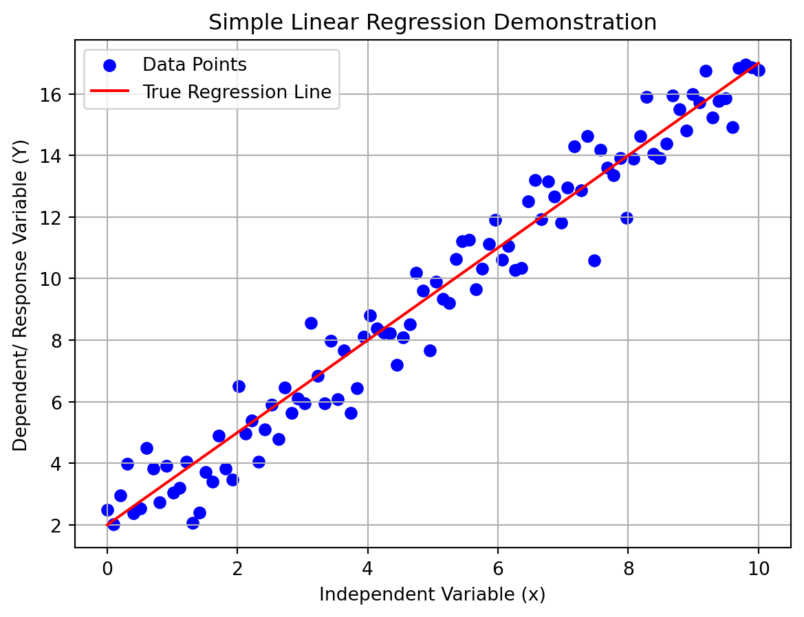
import numpy as npimport matplotlib.pyplot as plt# Set random seed for reproducibilitynp.random.seed(42)# Parameters for the linear regression modelalpha =2.0# Interceptbeta =1.5# Slopenum_samples =100# Number of data points# Generate synthetic datax = np.linspace(0, 10, num_samples) # Independent variable (input)e = np.random.normal(0, 1, num_samples) # Random error with mean 0Y = alpha + beta * x + e # Dependent variable (response)# Plot the data pointsplt.scatter(x, Y, color='blue', label='Data Points')# Plot the true regression line (without error)plt.plot(x, alpha + beta * x, color='red', label='True Regression Line')# Add labels and titleplt.xlabel('Independent Variable (x)')plt.ylabel('Dependent/ Response Variable (Y)')plt.title('Simple Linear Regression Demonstration')plt.legend()# Show the plotplt.grid(True)plt.show()
5.1.1 Least Squares Estimators Of The Regression Parameters
As mentioned previouslly, a simple linear regression model assumes a linear relationship between the mean response and a single independent variable.
It is expressed as: \[
Y = \alpha + \beta x + e
\]
\(x\) is the value of the independent variable (also called the input level).
\(Y\) is the response.
\(e\) represents the random error, assumed to be a random variable with mean \(0\).
Suppose the responses \(Y_i\) corresponding to the input values \(x_i\) for \(i = 1, \dots, n\) are observed and used to estimate \(\alpha\) and \(\beta\) in a simple linear regression model.
Let \(A\) be the estimator of \(\alpha\) and \(B\) be the estimator of \(\beta\).
The estimated response for the input \(x_i\) is \(A + Bx_i\).
The difference between the actual response \(Y_i\) and the estimated response is \((Y_i - A - Bx_i)\) is called residual.
The sum of squares of residuals or residual sum of squares (SSR) is given by: \[
SSR = \sum_{i=1}^n (Y_i - A - Bx_i)^2
\]
The method of least squares chooses \(A\) and \(B\) to minimize \(SSR\).
To find the minimizing values, differentiate \(SSR\) with respect to \(A\) and \(B\): \[
\frac{\partial SSR}{\partial A} = -2 \sum_{i=1}^n (Y_i - A - Bx_i)
\]\[
\frac{\partial SSR}{\partial B} = -2 \sum_{i=1}^n x_i (Y_i - A - Bx_i)
\]
Setting the partial derivatives to zero yields the normal equations: \[
\sum_{i=1}^n Y_i = nA + B \sum_{i=1}^n x_i
\]\[
\sum_{i=1}^n x_i Y_i = A \sum_{i=1}^n x_i + B \sum_{i=1}^n x_i^2
\]
Let \(\overline{Y} = \frac{\sum_{i=1}^n Y_i}{n}\) and \(\overline{x} = \frac{\sum_{i=1}^n x_i}{n}\).
The first normal equation can be rewritten as: \[
A = \overline{Y} - B \overline{x}
\tag{5.3}\]
Substituting \(A = \overline{Y} - B \overline{x}\) into the second normal equation: \[
\sum_{i=1}^n x_i Y_i = (\overline{Y} - B \overline{x}) n \overline{x} + B \sum_{i=1}^n x_i^2
\]
Simplifying: \[
B \left( \sum_{i=1}^n x_i^2 - n \overline{x}^2 \right) = \sum_{i=1}^n x_i Y_i - n \overline{x} \overline{Y}
\]
Solving for \(B\):
\[
B = \frac{\sum_{i=1}^n x_i Y_i - n \overline{x} \overline{Y}}{\sum_{i=1}^n x_i^2 - n \overline{x}^2}
\]
Using Equation 5.3 and the fact that \(n \overline{x} = \sum_{i=1}^n x_i\), we obtain the estimators for \(\alpha\) and \(\beta\).
Least Squares Estimators
The least squares estimators of \(\beta\) and \(\alpha\) for the data set \((x_i, Y_i)\), where \(i = 1, \dots, n\), are given by:
The estimator for \(\beta\) (\(B\)): \[
B = \frac{\sum_{i=1}^n x_i Y_i - \overline{x} \sum_{i=1}^n Y_i}{\sum_{i=1}^n x_i^2 - n \overline{x}^2}
\]
The estimator for \(\alpha\) (\(A\)): \[
A = \overline{Y} - B \overline{x}
\]
Here:
\(\overline{x} = \frac{\sum_{i=1}^n x_i}{n}\) is the mean of the independent variable \(x\).
\(\overline{Y} = \frac{\sum_{i=1}^n Y_i}{n}\) is the mean of the dependent variable \(Y\).
Problem
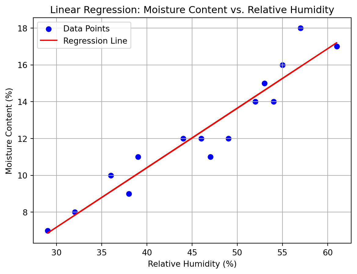
The raw material used in the production of a certain synthetic fiber is stored in a location without humidity control. Measurements of the relative humidity in the storage location and the moisture content of a sample of the raw material were taken over 15 days, resulting in the following data (in percentages):
Relative Humidity (%)
46
53
29
61
36
39
47
49
52
38
55
32
57
54
44
Moisture Content (%)
12
15
7
17
10
11
11
12
14
9
16
8
18
14
12
Use linear regression to express moisture content as a function of the relative humidity.
The Coefficient of Determination and the Sample Correlation Coefficient
Suppose we want to measure the amount of variation in the set of response values \(Y_1, \dots, Y_n\) corresponding to the input values \(x_1, \dots, x_n\).
A standard measure of variation in statistics is given by: \[
SST = \sum_{i=1}^n (Y_i - \overline{Y})^2
\]
(‘SST’ also refers to ‘Total Sum of Squares’)
Here, \(\overline{Y} = \frac{\sum_{i=1}^n Y_i}{n}\) is the mean of the response values.
If all \(Y_i\) are equal (i.e., \(Y_i = \overline{Y}\) for all \(i\)), then \(SST = 0\).
The variation in the response values \(Y_i\) arises from two factors:
Different input values: The input values \(x_i\) are different, leading to different mean values for the responses \(Y_i\).
Inherent variance: Even after accounting for the input values, each response \(Y_i\) has a variance \(\sigma^2\) and will not exactly equal the predicted value at its input \(x_i\).
To determine how much variation is due to the different input values and how much is due to inherent variance, consider:
The quantity: \[
SSR = \sum_{i=1}^n (Y_i - A - Bx_i)^2
\]
measures the remaining variation in the response values after accounting for the input values.
The difference: \[
SST - SSR
\]
represents the variation in the response values explained by the different input values.
The coefficient of determination (\(R^2\)) is defined as the proportion of the total variation in the response values that is explained by the input values: \[
R^2 = \frac{SST - SSR}{SST}
\]
\(R^2\) ranges from 0 to 1.
An \(R^2\) value of 1 indicates that the regression model perfectly explains the variation in the response values.
An \(R^2\) value of 0 indicates that the regression model does not explain any of the variation in the response values.
The sample correlation coefficient (\(r\)) measures the strength and direction of the linear relationship between the independent variable \(x\) and the dependent variable \(Y\): \[
r = \frac{\sum_{i=1}^n (x_i - \overline{x})(Y_i - \overline{Y})}{\sqrt{\sum_{i=1}^n (x_i - \overline{x})^2 \sum_{i=1}^n (Y_i - \overline{Y})^2}} = \sqrt{R^2}
\]
Note that the sign of r is the sign of B.
\(r\) ranges from -1 to 1.
An \(r\) value of 1 indicates a perfect positive linear relationship.
An \(r\) value of -1 indicates a perfect negative linear relationship.
An \(r\) value of 0 indicates no linear relationship.
Problem
Find the coefficient of determination and the sample correlation coefficient of the previous regression problem.
import numpy as npfrom sklearn.linear_model import LinearRegressionfrom sklearn.metrics import r2_scoreimport matplotlib.pyplot as plt# Data for relative humidity and moisture content humidity = np.array([46, 53, 29, 61, 36, 39, 47, 49, 52, 38, 55, 32, 57, 54, 44]).reshape(-1, 1) moisture = np.array([12, 15, 7, 17, 10, 11, 11, 12, 14, 9, 16, 8, 18, 14, 12])# Fit the linear regression model model = LinearRegression().fit(humidity, moisture)# Print the coefficientsprint(f"Intercept: {model.intercept_}")print(f"Coefficient: {model.coef_[0]}")# Predict the moisture content moisture_pred = model.predict(humidity)# Calculate the coefficient of determination (R^2) R_squared = r2_score(moisture, moisture_pred)print(f"Coefficient of Determination (R^2): {R_squared}")# Calculate the sample correlation coefficient (r) correlation_coefficient = np.sqrt(R_squared)print(f"Sample Correlation Coefficient (r): {correlation_coefficient}")# Plot the data points plt.scatter(humidity, moisture, color='blue', label='Data Points')# Plot the regression line plt.plot(humidity, moisture_pred, color='red', label='Regression Line')# Add labels and title plt.xlabel('Relative Humidity (%)') plt.ylabel('Moisture Content (%)') plt.title('Linear Regression: Moisture Content vs. Relative Humidity') plt.legend()# Show the plot plt.grid(True) plt.show()
In most applications, the response \(Y\) of an experiment is better predicted using multiple independent input variables rather than a single one.
A typical scenario involves \(k\) input variables, and the response \(Y\) is related to them by the equation: \[
Y = \beta_0 + \beta_1 x_1 + \beta_2 x_2 + \cdots + \beta_k x_k + e
\]
where:
\(x_j\) is the level of the \(j^{th}\) input variable (\(j = 1, \dots, k\)),
\(e\) is a random error term, assumed to be normally distributed with mean \(0\) and constant variance \(\sigma^2\).
Parameters:
The parameters \(\beta_0, \beta_1, \dots, \beta_k\) and \(\sigma^2\) are unknown and must be estimated from the data.
The data consists of observed values \(Y_1, Y_2, \dots, Y_n\), where each \(Y_i\) corresponds to a set of input levels \(x_{i1}, x_{i2}, \dots, x_{ik}\).
Expected Value:
The expected value of \(Y_i\) is given by: \[
E[Y_i] = \beta_0 + \beta_1 x_{i1} + \beta_2 x_{i2} + \cdots + \beta_k x_{ik}
\]
Determining the Least Squares Estimators
Least Squares Estimation:
Let \(B_0, B_1, \dots, B_k\) denote estimators of \(\beta_0, \beta_1, \dots, \beta_k\).
The sum of squared differences between the observed \(Y_i\) and their estimated expected values is: \[
\sum_{i=1}^n (Y_i - B_0 - B_1 x_{i1} - B_2 x_{i2} - \cdots - B_k x_{ik})^2
\]
The least squares estimators are the values of \(B_0, B_1, \dots, B_k\) that minimize the above sum of squared differences.
Method:
To determine the least squares estimators \(B_0, B_1, \dots, B_k\), we take partial derivatives of the sum of squared differences with respect to each estimator:
First, with respect to \(B_0\),
Then, with respect to \(B_1\),
And so on, up to \(B_k\).
By setting these partial derivatives equal to \(0\), we obtain a system of \(k + 1\) equations.
5.1.4 Matrix Representation of Multiple Regression
\(\beta\) be the parameter vector: \[
\beta = \begin{bmatrix}
\beta_0 \\
\beta_1 \\
\vdots \\
\beta_k
\end{bmatrix}
\]
\(e\) be the error vector: \[
e = \begin{bmatrix}
e_1 \\
e_2 \\
\vdots \\
e_n
\end{bmatrix}
\]
Dimensions:
\(Y\) is an \(n \times 1\) matrix (response vector),
\(X\) is an \(n \times p\) matrix (design matrix), where \(p = k + 1\),
\(\beta\) is a \(p \times 1\) matrix (parameter vector),
\(e\) is an \(n \times 1\) matrix (error vector).
Multiple Regression Model:
The multiple regression model can be written in matrix form as: \[
Y = X \beta + e
\]
Least Squares Estimators:
Let \(B\) be the matrix of least squares estimators: \[
B = \begin{bmatrix}
B_0 \\
B_1 \\
\vdots \\
B_k
\end{bmatrix}
\]
The normal equations can be written in matrix form as: \[
X^T Y = X^T X B
\] where:
\(X^T\) is the transpose of the design matrix \(X\),
\(X^T X\) is a \(p \times p\) matrix,
\(X^T Y\) is a \(p \times 1\) vector.
Solution:
The least squares estimators \(B\) can be obtained by solving the matrix equation: \[
B = (X^T X)^{-1} X^T Y
\] where \((X^T X)^{-1}\) is the inverse of the matrix \(X^T X\).
Residuals and Sum of Squared Residuals (SSR)
Residuals:
Let \(r_i\) denote the \(i^{th}\) residual, which is the difference between the observed response \(Y_i\) and the predicted value from the regression model: \[
r_i = Y_i - B_0 - B_1 x_{i1} - B_2 x_{i2} - \cdots - B_k x_{ik}, \quad i = 1, \dots, n
\]
The residual vector\(r\) is defined as: \[
r = \begin{bmatrix}
r_1 \\
r_2 \\
\vdots \\
r_n
\end{bmatrix}
\]
In matrix notation, the residual vector can be expressed as: \[
r = Y - XB
\] where:
\(Y\) is the response vector,
\(X\) is the design matrix,
\(B\) is the matrix of least squares estimators.
Sum of Squared Residuals (SSR):
The sum of squared residuals (SSR) is given by: \[
SSR = \sum_{i=1}^n r_i^2
\]
In matrix notation, the SSR can be written as: \[
SSR = r^T r
\] where \(r^T\) is the transpose of the residual vector \(r\).
Substituting \(r = Y - XB\), we get: \[
SSR = (Y - XB)^T (Y - XB)
\]
Expanding the matrix product: \[
SSR = [Y^T - (XB)^T](Y - XB)
\]
\[
SSR = Y^T Y - Y^T XB - B^T X^T Y + B^T X^T XB
\]
Simplification Using Normal Equations:
From the normal equations, we know: \[
X^T XB = X^T Y
\]
Substituting this into the expression for SSR: \[
SSR = Y^T Y - Y^T XB - B^T X^T Y + B^T X^T XB
\]\[
SSR = Y^T Y - Y^T XB
\] (since \(B^T X^T Y = B^T X^T XB\) from the normal equations).
Transpose Property:
Since \(Y^T XB\) is a scalar (a \(1 \times 1\) matrix), it is equal to its transpose: \[
Y^T XB = (Y^T XB)^T = B^T X^T Y
\]
Therefore, the expression for SSR simplifies further to: \[
SSR = Y^T Y - B^T X^T Y
\]
Final Computational Formula for SSR:
The sum of squared residuals (SSR) can be computed using the formula: \[
SSR = Y^T Y - B^T X^T Y
\]
This formula is computationally efficient but requires careful handling to avoid roundoff errors.
Interpretation:
The term \(Y^T Y\) represents the total variation in the response variable \(Y\).
The term \(B^T X^T Y\) represents the explained variation by the regression model.
The difference \(Y^T Y - B^T X^T Y\) gives the unexplained variation (SSR), which is minimized in the least squares method.
Coefficient of Multiple Determination (\(R^2\))
Definition:
The coefficient of multiple determination, denoted by \(R^2\), measures the proportion of the total variation in the response variable \(Y\) that is explained by the regression model.
It is defined as: \[
R^2 = 1 - \frac{SSR}{\sum_{i=1}^n (Y_i - \overline{Y})^2}
\] where:
\(SSR\) is the sum of squared residuals (unexplained variation),
\(\sum_{i=1}^n (Y_i - \overline{Y})^2\) is the total sum of squares (SST) (total variation in \(Y\)),
\(\overline{Y}\) is the mean of the observed response values \(Y_i\).
Range of \(R^2\):
\(R^2\) ranges between \(0\) and \(1\):
\(R^2 = 0\): The regression model explains none of the variation in \(Y\).
\(R^2 = 1\): The regression model explains all of the variation in \(Y\).
Formula in Terms of SST and SSR:
The formula for \(R^2\) can also be written as: \[
R^2 = \frac{SST - SSR}{SST}
\]
where:
\(SST = \sum_{i=1}^n (Y_i - \overline{Y})^2\) is the total sum of squares,
\(SSR = \sum_{i=1}^n (Y_i - \hat{Y}_i)^2\) is the sum of squared residuals.
Usefulness:
\(R^2\) is a useful measure of the goodness of fit of the regression model.
A higher \(R^2\) indicates that the model explains a larger proportion of the variation in the response variable \(Y\).
### Probabilistic Perspective of Linear Regression
Overview:
Linear regression can also be viewed from a probabilistic perspective.
In this view, the response variable \(Y\) is considered a random variable with a probability distribution that depends on the input variables \(x_1, x_2, \dots, x_r\).
Assumptions:
The response variable \(Y\) is normally distributed with mean \(\mu_Y\) and variance \(\sigma^2\).
The mean \(\mu_Y\) is a linear function of the input variables: \[
\mu_Y = \beta_0 + \beta_1 x_1 + \beta_2 x_2 + \dots + \beta_r x_r
\]
The variance \(\sigma^2\) is constant and does not depend on the input variables.
Model:
The linear regression model can be written as: \[
Y = \beta_0 + \beta_1 x_1 + \beta_2 x_2 + \dots + \beta_r x_r + \epsilon
\] where \(\epsilon\) is a random error term that follows a normal distribution with mean \(0\) and variance \(\sigma^2\): \[
\epsilon \sim N(0, \sigma^2)
\]
Likelihood Function:
Given a set of observed data points \((x_i, Y_i)\) for \(i = 1, \dots, n\), the likelihood function represents the probability of observing the data given the parameters \(\beta_0, \beta_1, \dots, \beta_r\) and \(\sigma^2\).
The likelihood function is given by: \[
L(\beta_0, \beta_1, \dots, \beta_r, \sigma^2) = \prod_{i=1}^n \frac{1}{\sqrt{2 \pi \sigma^2}} \exp \left( -\frac{(Y_i - \beta_0 - \beta_1 x_{i1} - \dots - \beta_r x_{ir})^2}{2 \sigma^2} \right)
\]
Log-Likelihood Function:
The log-likelihood function is the natural logarithm of the likelihood function: \[
\log L(\beta_0, \beta_1, \dots, \beta_r, \sigma^2) = -\frac{n}{2} \log (2 \pi \sigma^2) - \frac{1}{2 \sigma^2} \sum_{i=1}^n (Y_i - \beta_0 - \beta_1 x_{i1} - \dots - \beta_r x_{ir})^2
\]
Maximum Likelihood Estimation (MLE):
The parameters \(\beta_0, \beta_1, \dots, \beta_r\) and \(\sigma^2\) can be estimated by maximizing the log-likelihood function.
The maximum likelihood estimators (MLEs) of \(\beta_0, \beta_1, \dots, \beta_r\) are the same as the least squares estimators.
The MLE of \(\sigma^2\) is given by: \[
\hat{\sigma}^2 = \frac{1}{n} \sum_{i=1}^n (Y_i - \hat{Y}_i)^2
\] where \(\hat{Y}_i = \hat{\beta}_0 + \hat{\beta}_1 x_{i1} + \dots + \hat{\beta}_r x_{ir}\) are the predicted values from the regression model.
Inference:
The probabilistic perspective allows for statistical inference about the regression parameters.
Confidence intervals and hypothesis tests can be constructed for the parameters \(\beta_0, \beta_1, \dots, \beta_r\) and \(\sigma^2\).
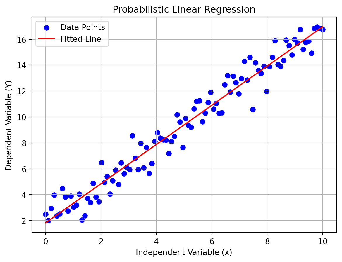
import numpy as npfrom scipy.stats import norm# Generate synthetic data np.random.seed(42) n =100 x = np.linspace(0, 10, n) beta_0 =2.0 beta_1 =1.5 sigma =1.0 epsilon = np.random.normal(0, sigma, n) Y = beta_0 + beta_1 * x + epsilon# Maximum Likelihood Estimation (MLE) for beta_0, beta_1, and sigma^2 X = np.vstack([np.ones(n), x]).T beta_hat = np.linalg.inv(X.T @ X) @ X.T @ Y Y_hat = X @ beta_hat sigma_hat = np.sqrt(np.sum((Y - Y_hat) **2) / n)print(f"Estimated beta_0: {beta_hat[0]}")print(f"Estimated beta_1: {beta_hat[1]}")print(f"Estimated sigma^2: {sigma_hat **2}")# Plot the data and the fitted lineimport matplotlib.pyplot as plt plt.scatter(x, Y, color='blue', label='Data Points') plt.plot(x, Y_hat, color='red', label='Fitted Line') plt.xlabel('Independent Variable (x)') plt.ylabel('Dependent Variable (Y)') plt.title('Probabilistic Linear Regression') plt.legend() plt.grid(True) plt.show()
Logistic regression is used when the response variable is categorical, typically binary (0 or 1).
It models the probability that a given input point belongs to a particular category.
Logistic Function:
The logistic function (also called the sigmoid function) is used to model the probability: \[
P(Y = 1 \mid \mathbf{x}) = \frac{1}{1 + \exp(-(\beta_0 + \beta_1 x_1 + \beta_2 x_2 + \dots + \beta_r x_r))}
\]
Logistic Regression Model:
The logistic regression model can be written as: \[
\log \left( \frac{P(Y = 1 \mid \mathbf{x})}{1 - P(Y = 1 \mid \mathbf{x})} \right) = \beta_0 + \beta_1 x_1 + \beta_2 x_2 + \dots + \beta_r x_r
\]
Here, the left-hand side is the log-odds (logit) of the probability of the response being 1.
Estimation of Parameters:
The parameters \(\beta_0, \beta_1, \dots, \beta_r\) are estimated using the method of maximum likelihood.
The likelihood function for logistic regression is given by: \[
L(\beta_0, \beta_1, \dots, \beta_r) = \prod_{i=1}^n P(Y_i \mid \mathbf{x}_i)^{Y_i} (1 - P(Y_i \mid \mathbf{x}_i))^{1 - Y_i}
\]
Log-Likelihood Function:
The log-likelihood function is: \[
\log L(\beta_0, \beta_1, \dots, \beta_r) = \sum_{i=1}^n \left[ Y_i \log P(Y_i \mid \mathbf{x}_i) + (1 - Y_i) \log (1 - P(Y_i \mid \mathbf{x}_i)) \right]
\]
Fitting the Model:
The parameters are estimated by maximizing the log-likelihood function using numerical optimization techniques.
Checking the goodness of fit
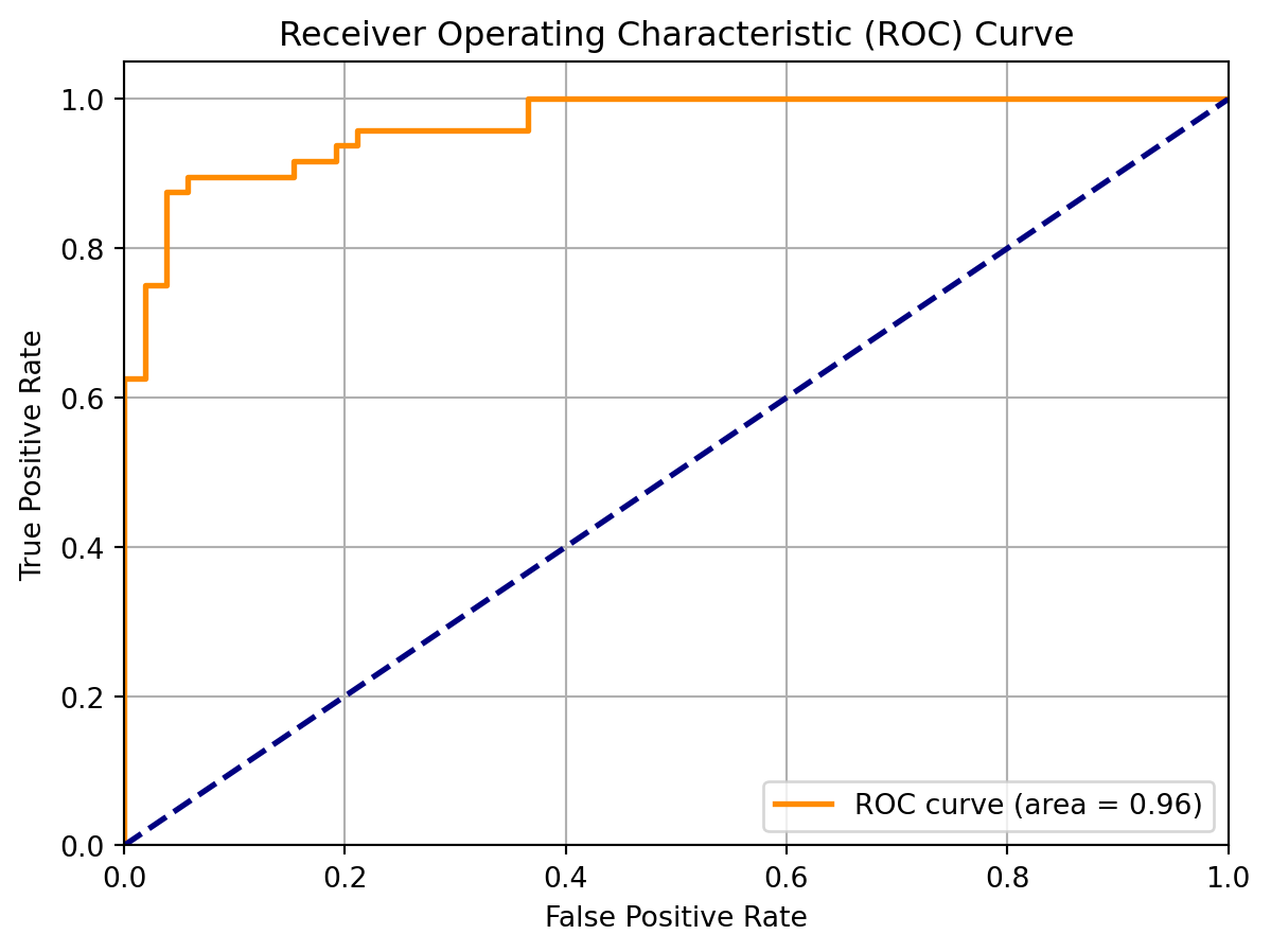
5.2.1 Confusion Matrix, Accuracy, and ROC Curve
Confusion Matrix:
A confusion matrix is a table used to evaluate the performance of a classification model.
It summarizes the counts of true positive (TP), true negative (TN), false positive (FP), and false negative (FN) predictions.
The matrix helps in understanding the types of errors the model is making.
Accuracy:
Accuracy is a metric that measures the proportion of correct predictions made by the model.
It is calculated as the sum of true positives and true negatives divided by the total number of predictions: \[
\text{Accuracy} = \frac{TP + TN}{TP + TN + FP + FN}
\]
While accuracy is a useful metric, it may not be sufficient for imbalanced datasets where one class is more frequent than the other.